
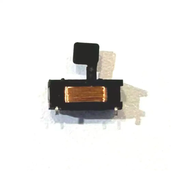
1. Wafer-Level Packaging Set a New Brief for Small Shutters
Wafer-level packaging (WLP) cut the cost and size of uncooled infrared detectors by a step change, and in doing so created an entire category: sub-$200 handheld thermal imagers and pocket-sized industrial thermometers. But WLP did not only deliver “cheaper and smaller.” It placed three new constraints on the NUC shutter:
- Less room. A smaller detector means less clearance left for the shutter in the optical bench. In a handheld camera engine, a few millimetres is all the shutter gets.
- Faster drift. To cut cost and volume, these engines generally omit TEC stabilisation. Without temperature control, the detector substrate tracks ambient, and non-uniformity drifts faster and further — so calibration must happen more often.
- Tighter cost. Once the end product price drops, the shutter’s cost, assembly labour and drive-circuit complexity all get re-examined.
A 9.8 × 4 × 3.7 mm single-blade shutter for 256×192 wafer-level detectors is the engineering answer to all three at once.
2. Key Specifications
| Item | Specification |
|---|---|
| Outer dimension | 9.8 × 4 × 3.7 mm |
| Mechanism | Single-blade type |
| Blade material | Metal, matte (anti-reflection) coated |
| Blade size | 3.5 × 3.0 mm |
| Detector compatibility | 256×192 wafer-level infrared detectors |
| Drive | Monostable solenoid |
| Action logic | Energised = open / de-energised = closed |
| Drive voltage | 3.0 – 3.3 V |
| Actuation life | 1,000,000 cycles |
| Mounting | DIP plug-in (through-hole PCB) |
| Typical applications | Handheld thermal imagers, industrial thermometers |
3. The 3.5 × 3.0 mm Blade: A Coverage Problem You Have to Do the Maths On
First, the blade has to cover the detector
The blade size is not a number that stands alone — it must fully cover the detector’s active area, with margin. For a 256×192 array:
| Pixel pitch | Active area | Coverage, 3.5 mm (X) | Coverage, 3.0 mm (Y) |
|---|---|---|---|
| 17 µm | 4.35 × 3.26 mm | ✗ insufficient | ✗ insufficient |
| 12 µm | 3.07 × 2.30 mm | ✓ +14% margin | ✓ +30% margin |
| 10 µm | 2.56 × 1.92 mm | ✓ +37% margin | ✓ +56% margin |
| 8 µm | 2.05 × 1.54 mm | ✓ +71% margin | ✓ +95% margin |
So a 3.5 × 3.0 mm blade maps precisely onto 256×192 wafer-level detectors at 12 µm pitch and below — which is exactly where WLP devices live.
The real margin killer is the incident cone
That table only accounts for the active area, and that is not enough. The shutter sits in front of the detector, and what lands on the blade is not a parallel beam — it is a cone converging from the lens. The projected beam diameter at the blade plane is:
\begin{aligned}
D_{\text{blade, required}}= D_{\text{active}} + 2\,d\,\tan\theta,
\tan\theta= \frac{1}{2N}
\end{aligned}
where d is the blade-to-detector gap and N is the lens f-number. In other words, the gap between blade and detector magnifies the cone: the faster the lens and the larger the gap, the larger the blade must be.
Take 12 µm / 256×192 (active width 3.072 mm). The blade has only 0.214 mm of margin per side in X, which caps the allowable gap at:
| Lens f-number | Half-cone \tan\theta | Max allowable gap d |
|---|---|---|
| f/1.0 | 0.500 | 0.43 mm |
| f/1.2 | 0.417 | 0.51 mm |
| f/1.4 | 0.357 | 0.60 mm |
| f/1.6 | 0.313 | 0.69 mm |
| f/2.0 | 0.250 | 0.86 mm |
The Y axis has 0.348 mm per side and is correspondingly more forgiving, so X is the binding constraint.
This yields a clear design rule: in an f/1.0-class engine, the blade must sit hard against the detector — within roughly 0.5 mm — or edge pixels will still see part of the scene while the shutter is closed, and the reference is no longer uniform. If the mechanical stack cannot get that close, specify a larger blade or a slower lens.
4. Metal + Matte Coating: Getting “Uniform” in Both Temperature and Emissivity
NUC works by having every pixel look at a known, uniform target at the same moment. Any non-uniformity in that reference gets written into the correction coefficients, and every subsequent frame carries the error. Uniformity requires two things at once — and a metal blade delivers both.
Uniform temperature ← metal’s high thermal conductivity
The radiance a blade presents depends on its temperature. Metal conducts heat far better than plastic or film, so any local temperature variation across the blade is quickly levelled out and the whole blade radiates at essentially one temperature. This is difficult for organic film blades such as PET or polyimide: poor conduction leaves temperature gradients in place.
Uniform emissivity ← the matte coating
A polished metal surface has very low emissivity — it is close to a mirror, and will reflect the lens, the housing walls and even the scene into the detector, so the “uniform reference” arrives carrying an image of the scene. A metal blade therefore has to be matte-finished: a matte coating is a good absorber and, by Kirchhoff’s law, an equally good emitter, giving high and stable emissivity.
The critical word is uniform coating thickness. Vary the thickness and emissivity varies with position, so the corrected image acquires a fixed light-and-dark pattern that no later processing can remove.
What non-uniformity actually costs
An order-of-magnitude estimate: ambient 25 °C, blade at 40 °C (8–14 µm band). If emissivity varies by 2 % across the blade surface, the radiance difference the detector sees between two regions is about 0.43 % of total radiance. In the LWIR near 300 K, radiance changes with temperature at roughly 1.6 % per kelvin — which converts to an apparent temperature error of about 0.3 °C.
For an industrial thermometer specified at ±2 °C, that 0.3 °C is a material line item in the error budget. And that is only the non-uniformity term: if the blade additionally reflects the scene, the error grows further.
This is also why, across a 1,000,000-cycle life, coating adhesion and wear resistance are reliability specifications, not cosmetic ones. Once the coating wears or lifts locally, the emissivity distribution changes and the NUC baseline drifts with it.
5. Monostable Solenoid: Calibration Happens at Zero Coil Power
This shutter uses a monostable solenoid: energised to open, de-energised to close. That polarity choice has several knock-on benefits.
The coil is not generating heat while the reference is being measured
NUC requires the shutter to be closed, and closed is exactly the de-energised state. So at the moment the blade is measured as the reference surface, there is no current in the coil, no Joule heating, and the blade and housing are thermally quiet. If instead the shutter had to be held closed by energising it, the coil’s own dissipation would continuously disturb the reference temperature. This is the most easily overlooked — and most substantive — advantage of a monostable design in a NUC application.
Fail-safe by default
On power loss, brown-out or an MCU fault, the shutter returns to closed and the detector window is shielded — no direct exposure of the detector to strong light or dust. On a portable device that gets dropped, knocked and run to empty battery, that is a valuable default state.
The simplest possible drive
A monostable mechanism needs no reversal, so it needs no H-bridge and no polarity control logic. One low-side switch and one GPIO drive it, and the control sequence collapses to two states: on and off. Fewer parts, fewer failure points, less board area.
One trade-off to account for
Monostable operation means the coil must be continuously energised to hold the shutter open during imaging, so hold current is a critical parameter on a battery-powered handheld. Pull-in current for a solenoid is normally higher than hold current; confirm the hold current and duty-cycle capability with your supplier and budget for it in the system power envelope.
6. 3.0 – 3.3 V: Matching Both the Logic Rail and a Single Li-ion Cell
The 3.0 – 3.3 V window sits at the intersection of two industry defaults:
- It matches a 3.3 V logic rail. The shutter can run straight off the system’s 3.3 V digital supply — no level shifting, and no dedicated rail for the shutter.
- It overlaps a single Li-ion cell’s discharge range. Li-ion and Li-polymer cells operate across roughly 3.0 – 4.2 V, and 3.3 V falls in the middle-to-late part of that curve. In many power architectures the shutter can therefore run from the battery through simple regulation, with no boost converter.
Eliminating a switching stage removes not just cost and board area, but its switching noise as well. Inside a handheld thermal imager, a low-noise analogue front end, a very weak signal chain and a radio all share the same enclosure — every switching node on the supply is a potential interference source.
7. DIP Plug-In Mounting: Making Mechanical Fixing and Electrical Connection One Thing
In a 9.8 mm envelope, any additional bracket, screw or connector is a luxury. DIP plug-in mounting collapses two problems into one: the pins serve simultaneously as the electrical connection and the mechanical fixing.
| Benefit | What it means in practice |
|---|---|
| No separate hardware | No bracket, no screws — and therefore no assembly labour, part cost or tolerance stack to go with them. |
| Drop and vibration resistance | A through-hole solder joint retains far better than surface mount, which is the more dependable choice for a handheld device that is carried, gripped and occasionally dropped. |
| Locating accuracy comes from the PCB | Pin holes and detector pads are positioned on the same board by the same process, so optical-axis alignment is set by tooling rather than by operator judgement during assembly. |
| Thermal coupling | The pins tie the housing to the PCB copper, giving the housing a stable heat-spreading path that helps hold blade temperature steady. |
Integration notes: allow clearance for the blade’s travel in your layout, verify pin-hole positions against the detector’s optical axis for concentricity, and control the blade-to-detector gap as established in §3.
8. 1,000,000 Cycles: Converting to Years of Service
Because WLP engines drop temperature stabilisation, calibration frequency goes up — which makes life expectancy a qualification requirement in this category rather than a bonus. Converting 1,000,000 cycles to time:
| NUC interval | Duration covered by 1 M cycles (continuous) |
|---|---|
| 30 seconds | ≈ 0.95 years |
| 60 seconds | ≈ 1.9 years |
| 5 minutes | ≈ 9.5 years |
Even running continuously on an aggressive 30-second calibration strategy, a million cycles represents nearly a year of uninterrupted operation; at 60-second intervals it equates to many years of normal use. For the overwhelming majority of handheld thermal imagers and industrial thermometers, the shutter is no longer the limiting component in the product’s life.
Two caveats
- Life figures are sensitive to drive voltage, actuation frequency and ambient temperature — confirm the actual test conditions with your supplier during selection.
- On a handheld device, actuation count reflects real shutter wear far better than operating hours, so plan maintenance by cycle count.
9. Typical Applications
- Handheld thermal imagers. Space is measured in millimetres, and the 9.8 × 4 × 3.7 mm body leaves room for optics and the main board; 3.3 V direct drive removes a power rail; through-hole mounting survives daily handling and drops; and 1,000,000 cycles covers the high calibration rate of an unstabilised engine.
- Industrial thermometers. Measurement accuracy depends directly on the quality of the NUC reference, and the metal blade plus matte coating delivers uniformity in both temperature and emissivity. For continuously operating instruments, the monostable hold current must be included in the power budget.
- Other applications. Micro camera engines, portable thermometry modules, and any compact infrared imaging system built on a 256×192 or smaller wafer-level detector.
10. Selection and Integration Checklist
- Do the coverage maths before fixing the gap. Verify blade size against the equation above, and note that X and Y margins are not equal.
- Confirm emissivity uniformity and coating durability. Request emissivity data and its spatial distribution, and confirm coating condition after 1,000,000 actuations.
- Confirm hold current and duty cycle — especially for battery-powered handhelds.
- Confirm drive timing and default state against the product’s fail-safe strategy.
- Confirm pin-hole positions, optical-axis concentricity and blade travel clearance.
- Confirm life test conditions and set the maintenance interval from them.
11. Conclusion
Wafer-level packaging brought infrared imaging into the handheld price band, and pushed the shutter into a tighter corner: less space, more frequent calibration, sharper cost pressure. A 9.8 × 4 × 3.7 mm body, a 3.5 × 3.0 mm matte-coated metal blade, zero-coil-power calibration from a monostable mechanism, 3.3 V direct drive, DIP plug-in mounting and a 1,000,000-cycle life each answer one of those constraints.
Developing a handheld thermal imager or an industrial thermometer? Send us your detector specification (pitch and active area), lens f-number and available clearance — our engineers will work through the blade coverage and gap calculation and recommend a model, with 2D/3D drawings available at quotation stage.
Web: www.ky-ele.com | Email: kuma@ky-ele.com